-Correct function of the MPP tracking algorithm

-Inverter stability

-Statistical frequency of the dynamic changes

Good devices achieve values over 99.1%.

Although a PV module’s temperature has a direct influence on the voltage and, therefore, the MPP tracking, it only marginally affects the MPP tracking speed due to the thermal mass of PV modules. The impact of the changing irradiation levels is also negligible if the changes occur to a minor extent--in other words, if the changes occur under a constantly clear sky at high levels and under constantly cloudy days at low levels.

The irradiation levels quickly change on clear days with clouds passing by. Changes between 300 W/m2 and 1,000 W/m2 do not significantly affect the MPP voltage. However, the transition from a lower to a higher irradiation level causes selective large and quick surges in the MPP voltage. Most of the MPP tracking procedures cannot follow these rapid changes. Over the course of a year, however, they only cause marginal yield reductions. Therefore, the tracking speed does not need to follow these rapid changes. In principle, a speed of approximately one percent of the MPP voltage per second is sufficient.

The adaptation efficiency affects a PV system’s yield. The MPP tracker operates more efficiently at somewhat slower speeds and correctly than when it operates faster and incorrectly.

Apart from high efficiencies, the inverter’s availability is a decisive quality criterion. It is commonly specified based on the failure rates--in more specific terms, the Mean Time Between Failures (MTBF). This rate specifies the period between two failures, which are not the result of component wear. A device’s service life is typically represented with a so-called ‘bathtub curve’

This curve describes the trend of the failure probabilities of components and devices. In the beginning, an increased amount of early failures are to be expected. They are caused by faulty components and manufacturing defects. They are usually prevented by burn-in and in-circuit tests, such as the ones KACO performs. During the statistical failure phase, the failure probability is only marginal. It has a value of λstat. The reciprocal value describes the MTBF. After this phase, the failure probabilities increase due to the increasing signs of wear. A device is considered to have exceeded its service life starting with a value of λX.

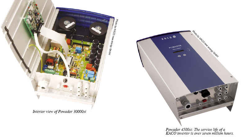
The MTBF is a statistical parameter and is specified in Failures In Time (FIT). It can be calculated or determined through field tests--but such tests are expensive. Determining the MTBF primarily depends on the ambient conditions for the respective component or device (current and voltage load and ambient temperature). In this case, there are various options for calculating the values. KACO uses the standards MIL-HDBK-217, SN 29500 and IEC62380 for this. The common factor of these three methods is that the MTBF for a complete device is determined from the sum of the MTBF values of all individual components. The respective basic data, which is defined from large-scale field tests conducted under reference conditions, forms the basis for calculating the values of the individual components. The values for an individual component under the specified conditions (temperature, voltage, and current) are determined from the conversion factors. The three specifications primarily vary in their underlying basic data that is acquired according to different criteria and their respective conversion factors. The calculations of the MTBF values for a KACO inverter, which are based on the specified standard values, yield a long service life totaling approximately 7,498,500 hours.

However, various research methods demonstrated somewhat severe differences between the applied procedures and the results showed significant deviations from one another. Therefore, theoretically determined values are not always reliable. In particular, several influencing factors, which are not included in the calculations, play a critical role in a PV inverter’s reliability. The device’s availability strongly depends on the conditions that are derived from the interplay with the other PV system components. For example, defects caused by faulty designs or failures resulting from external influences (e.g., overvoltages caused by lighting strikes) may occur. In addition, the lower quality components in a PV system affect an inverter’s failure probability.

The values derived from the calculations can provide an indication of a device’s quality. However, they are not significantly associated with inverter failures in real PV systems. The experiences from real systems are indispensable and offer valuable information on a device’s reliability.

 The inverters disconnect from the grid under certain grid conditions. In this case, the disconnection time in Germany is 180 seconds. Inverters disconnect from the grid relatively often in weak grids or if parameters are incorrectly set. An inverter that unnecessarily disconnects from the grid on an hourly basis results in yield losses of up to 8%. Therefore, the inverter must feature reliable and stable grid monitoring so that the device is only disconnected from the grid when it is actually necessary. KACO inverters operate with reliable algorithms that keep the frequency in which the inverters unnecessarily disconnect from the grid to a minimum. This significantly contributes to the high energy yields of PV systems.

An inverter should not be measured solely on its conversion efficiency. Instead, its rating should be based on the interplay of the aforementioned efficiencies and the high availability of the device or the entire PV system. In particular, the adaptation efficiency plays a vital role in high PV system yields.

The MTBF calculations, which allow theoretical conclusions to be drawn on a device’s failure probability, provide information of an inverter’s reliability. However, various methods produce significantly different information. In addition, numerous influencing factors that occur when a PV inverter is operating are not taken into consideration. Field data of real PV systems are more meaningful.

In contrast, inverters with very high efficiencies that consistently fail produce lower yields than devices that operate reliably. Therefore, a high availability and reliable monitoring in inverters are essential for high yields.

Dipl.-Ing. (FH) Martin Frick is Product Manager at KACO new energy (www. kaco-newenergy.com), responsible for the Powador XP series central inverters.